Of decomposing functions

Functions occupy a central position in the whole of mathematics, a linear transformation is a function, there are linear transformation on functions, there are vector spaces of functions, for every vector space there is a dual space which contains essentially functions. So much for functions that we come up with something more.
For those who dont want to read all that written below and and still know what the whole bussiness is about.Its this. Any function can be broken down into an infinite series of function which consists of only sines. And the accompanying diagram might help.
Now continue.
Since a vector space consists of vectors which know how to get added to another vector and they also know,when presented with a scalar from the field on which the vector space is defined,how to form a new vector which it such that their summation and scalar multiplication lies in the same space. Of course there are additional properties like commutativity of vectors,associativity, two distributive laws (one on vectors,other on scalars), existence of additive identity(equivalent of 0), additive inverse(negative of that vector) and multiplicative idenity.Note that there is no multiplicative inverse,which if added will also make the vector space a field.But we are here today to worry about vector spaces not field. Fields just provide scalars as components of the vectors in vector space.
Now we do not mention what might constitute the vectors in this space,we just provide the rules. As always,it comes with lot of freedom, you could have vectors which contains numbers (which might be real or complex depending on field), polynomials, tea/coffee (provided you define addition and multiplication for them) and most importantly functions.
Of course there is a twist here, since we are talking about infinite-dimensional spaces (at least the function space and the polynomial space which are not exactly the same),we do not know if it even makes sense to talk about some collection of numbers which we don't know anything about.And here the notion of inner product helps to define the criterion to be satisified by a collection of numbers to be called a member of the vector space(since here we are talking about functions, numbers can be read as functions where we arbitarily fix the domain).This is the idea behind so called Lp spaces, inner product is essentially a 2-norm, in the sense , length of a vector 'x' is Sqrt[(<x|x>)] which translates to a p-norm as (Summation xi^p)^(1/p) where xi are the components of the x vector.
Coming to the topic.
We know, any vector in the vector space can be written as linear combination of basis vectors.
I give you this, that sin(n Pi x/L) forms a basis for the function space L2 where L is the upper limit of the domain starting from 0(you could choose it to be anything). On top of that,this is an orthogonal basis meaning inner product of two random basis vectors will give zero,if they are not the same.
Now this means that i can represent any function as linear combination of
sin (n Pi x/L) .Ain't that cool?
Give me any arbitary even discontinous function and i will approximate it with these sines.
This is called the Fourier transformation and the coefficients form what is called the Fourier series.
Take an example.
We have a function f(x) = x
When we plot it,it is a straight line.

Now can this neat straight function be approximated by those oscillating sines, i mean ,can you get that annoyance.
Ok so here the fact, that n-th coefficient Cn of the basis function is given by the following formula

this can easily be derived from the fact that the basis functions are orthogonal and hence satisfy the following relation
Given any arbitary vector x
Expressing it in basis x= a1 b1 + a2 b2 +... + an bn where ai's belong to the field and bi's to the vector space.
taking inner product of x with bi
   <bi|x> = <bi|a1b1> + ... + <bi| an bn>
an comes out by the linearity property of bilinear forms(which inner product is).
               = a1<bi|b1> + ... +an <bi| bn>
now because of the orthogonality property <bi|bj> = <conjugate(ki)X(ki)
if i=j ,0 otherwise.
So <bi|x> = ai<bi|bi>
Hence ai = <bi|x>/ <bi|bi>, ai is the ith coefficient of the arbitary vector.Same principle applies to functions and hence we get our formula for coefficient of the function,except that inner product here is defined in terms of integrals over the limit of the domain of function on which decomposition is necessary.

<f(x)|g(x)> =

(Note that i am not sure if this domain can extend to infinity because sometimes the integral might not converge ,well in principle you can use a weighted inner product for that but for current purposes its not necessary).
Now that we know how to get the coefficients of the basis functions for the arbitary function (here f(x)=x).
Calculating Cn for the given function we get

  Note L=1,so the domain of the real valued function is [0,1]
Now everything is done, we know are basis vectors are of the form

except that we need to place our coefficient in front of them(t is same as x here).
Lets do that and see what we get.
For approximation with just 1 basis vector

For approximation with just 2 basis vector

For approximation with just 3 basis vector

We could go adding terms so that more an more terms get added,but how would we know that these are really the approximation.Well,nothing like plotting.
Serially plotting the approximating function along with the real function with adding more terms one by one

the last diagram was drawn using 10 terms.
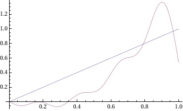
Notice that the approximation is getting better and better,although still not quite it.
How fast the infinite basis series converges to your arbiatry function depends on many factors like continuity,smoothness etc. Still you get the idea. dont you.

Also associated with Fourier decomposition is something known as Gibbs phenomenon ,not a big deal. ITs just that when you try to do Fourier decomp for discontinous functions,it will overshoot at the discontinuity and as you might think that these will die down upon adding more and more terms, well they do decrease but approach a finite limit .Guess this gives you a way of idenitifying functions from their Fourier decomps (its a joke if you dont get it).